No doubt, there are a lot of excellent commerical and academic packages for interactive, visible molecular dynamics simulations, but we strongly believe that it is better to understand your investigation tools by building it. The free software on the Internet and high-performance personal computer architecture provide us this opportunity.
According to our definition, virtual Laboratory is the use of computer's hardware and software to generate a simulation of an experiment. The basic requirements for a virtual laboratory should contain the following capabilities, visibility, interactivity, and high-performance computing. To achieve these requirements, it is important to know how to utilize and exploit the current computer technology. Thanks to the free software philosophy on the Internet, we can build our virtual laboratory from scratch by combining different sofeware components together which range from operating systems, programming languages, numerical libraries to application programs. The benefit of this approach is that we can modify the source codes of these software components to meet our need if it is necessary.
The virtual laboratory consists of four components: a computational engine, a display window, an instrument panel and a control panel.
The computational engine is used for generating the evolution of system and evaluating certain physical quantites such as temperature, pressure, total energy, kinetic energy etc. Then it sends these data to the display window and the instrument panel respectively.
The display window receives the system configuration from the computational engine and show them on the screen to generate an animation effect.
The instrument panel receives physical quantites from the computational engine and display them on the screen to provide a constant monitor of system status.
The control panel provides an interactive environment for simulations. Investigator can use it to change system's parameters such as volume, temperature and system's process such as quasi-static compression, free expansion etc in real time.
Putting these components together, a virtual laboratory can be built for the study of complex systems in an interactive way.
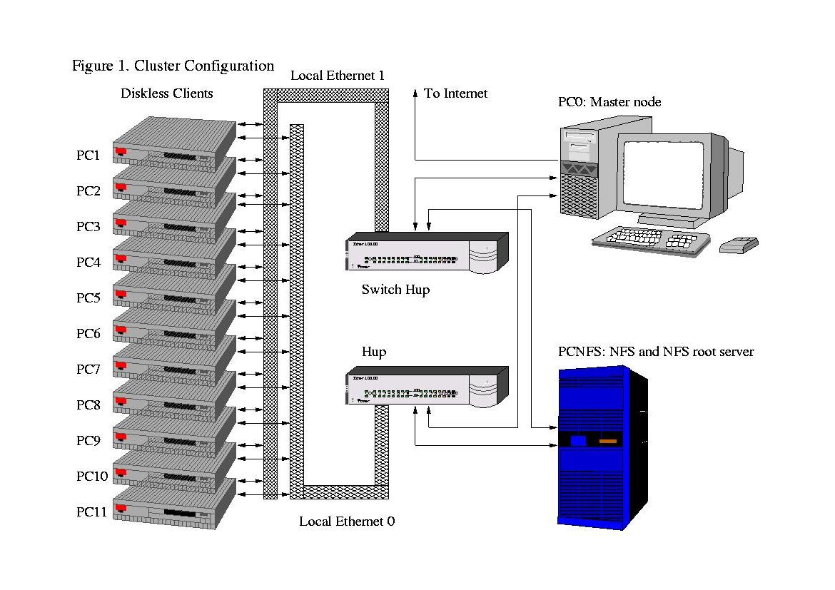
The hardware platform is a PC cluster with one master node, one NFS and NFS-root server node, and several diskless client nodes. All of these nodes are connected to switch hups by ethernet to achieve the parallel computing capability. The cluster hardware configuration is shown in Figure 1.
Two Pentium III 1GHz CPU, 512M RAM, three 3Com 3c905c ethernet cards, one 30G bytes hard disk, one floppy, one VGA card, one monitor
Two Pentium III 1GHz CPU, 512M RAM, two 3Com 3c905c ethernet cards, one 30G bytes hard disk, one floppy, one VGA card, one monitor
One Pentium III 1GHz CPU, 512M RAM, two 3Com 3c905c ethernet cards, no hard disk, one floppy, one VGA cards (for debugging)
D-Link DES-1016R, D-Link DFE-916DX
We use the following six examples to demonstrate what the virtual laboratory can be used for researchers.
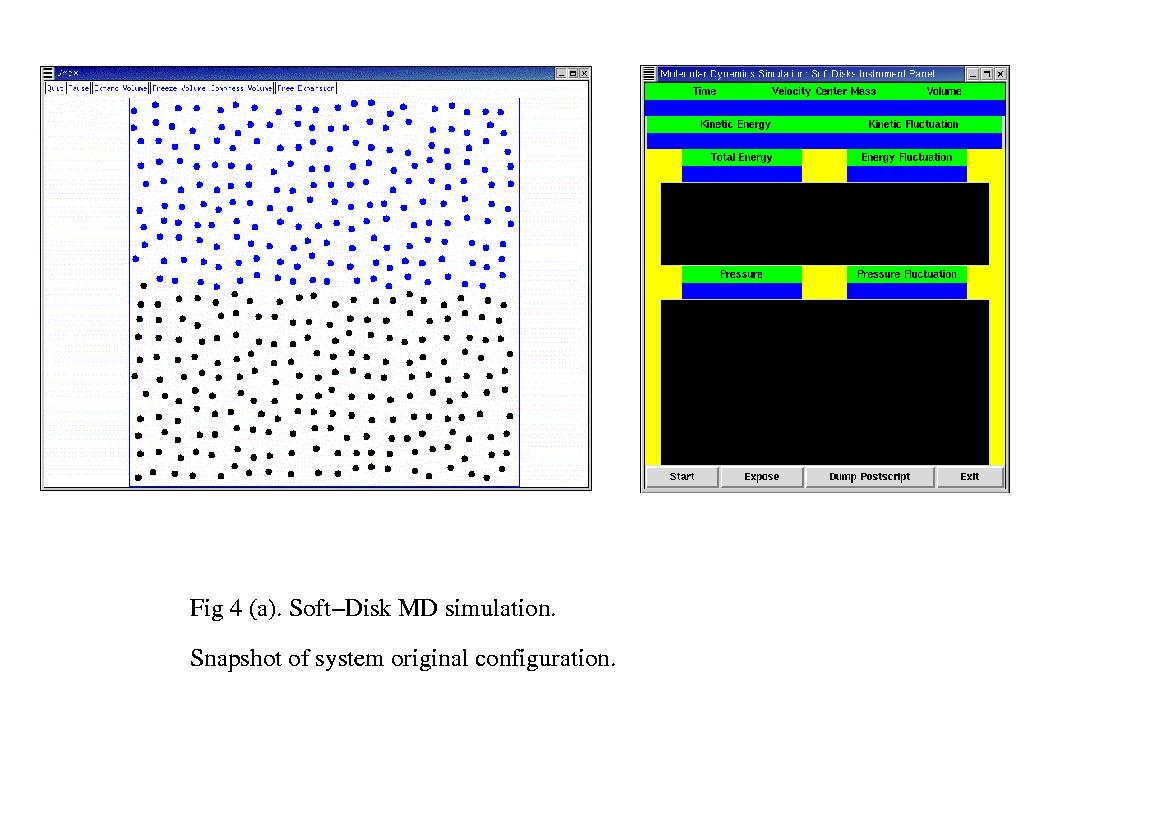
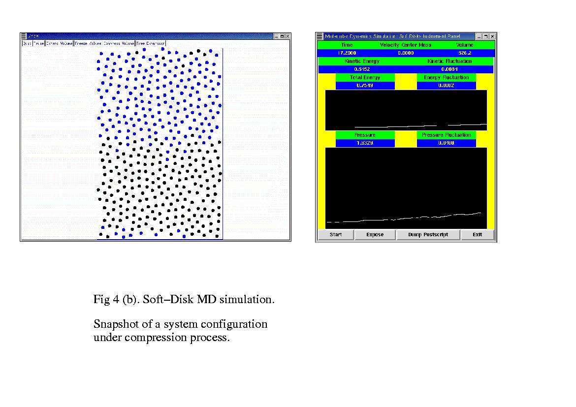
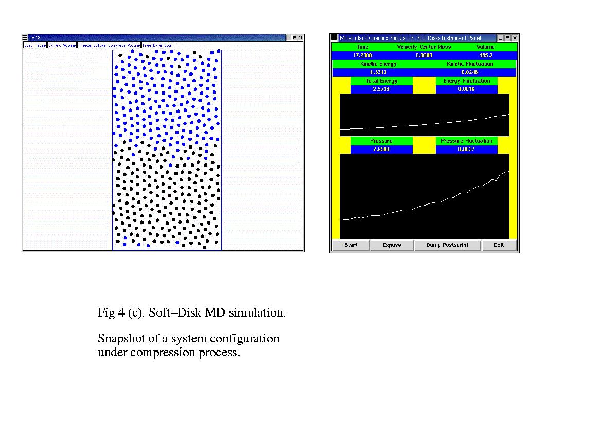
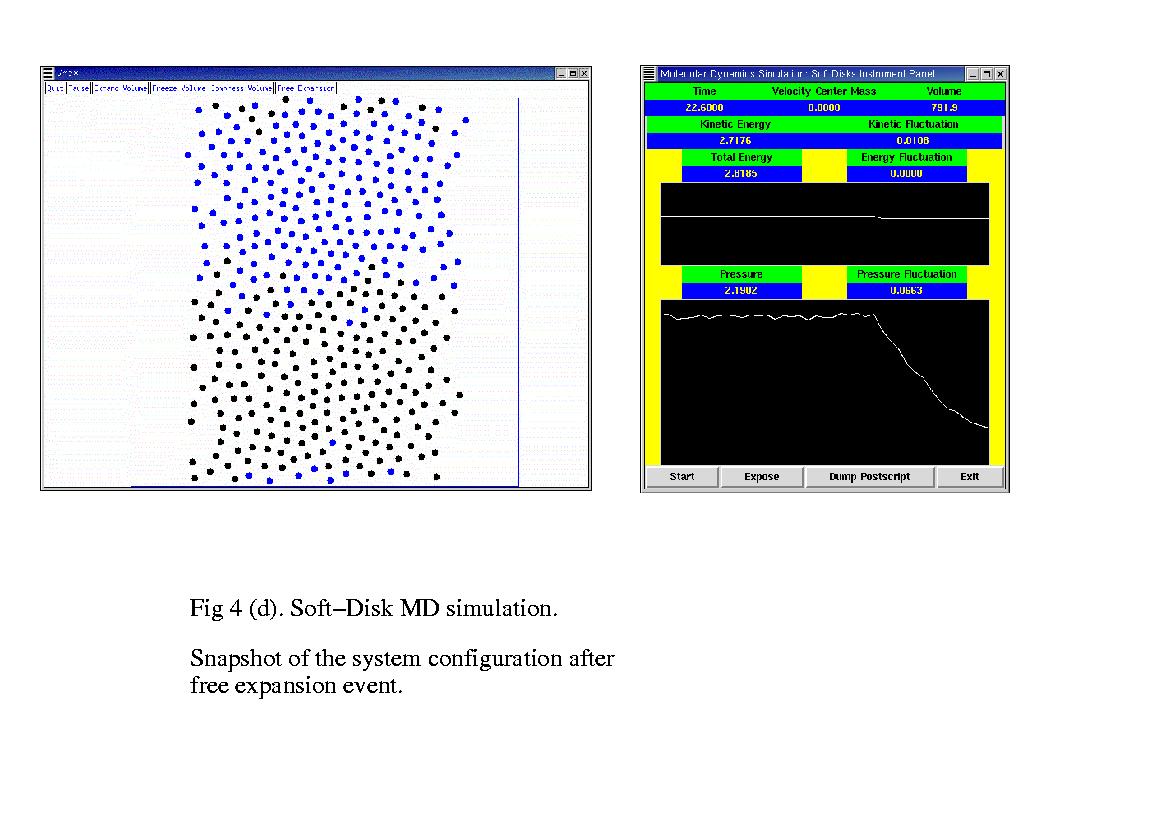
The major purpose of this example is used for the demonstration of the combination of different software components to perform an interactive simulation. The display window shows the evolution of the system. The control panel contains six events, "Quit", "Pause", "Expand Volume", "Compress Volume", and "Free Expansion" (Figure 4(a)). Each event can be invoked by mouse clicking and the system will response to the event accordingly. For example, if we click the "Compress Volume" event, we can see from the instrument panel that the pressure of the system is increasing (Figure 4(b), Figure 4(c) ). If we click the "Free Expansion" bottom, the system will undergo the free expansion process (Figure 4(d)). The instrument panel acts like some measurement gauges from which the kinetic energy, pressure, etc, of the system can be obtained.
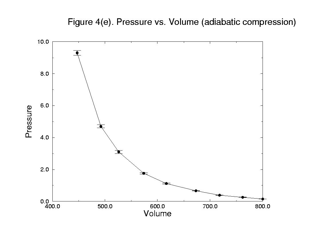
Using mouse-click to generate different events, for example, compression of the system. After the event been sent, we can see from instrument panel and display window that the various physical quantities are changing with simulation time.
We can stop this process at any time by sending freeze event and record the pressure and volume values after the system reaches equilibrium. Repeating the process several time, we can obtain a quasi-static adiabatic P-V diagram in Figure 4(e).
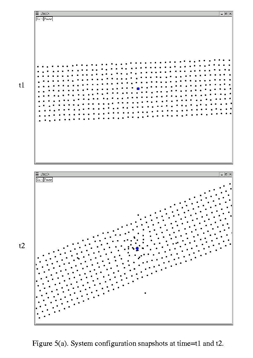
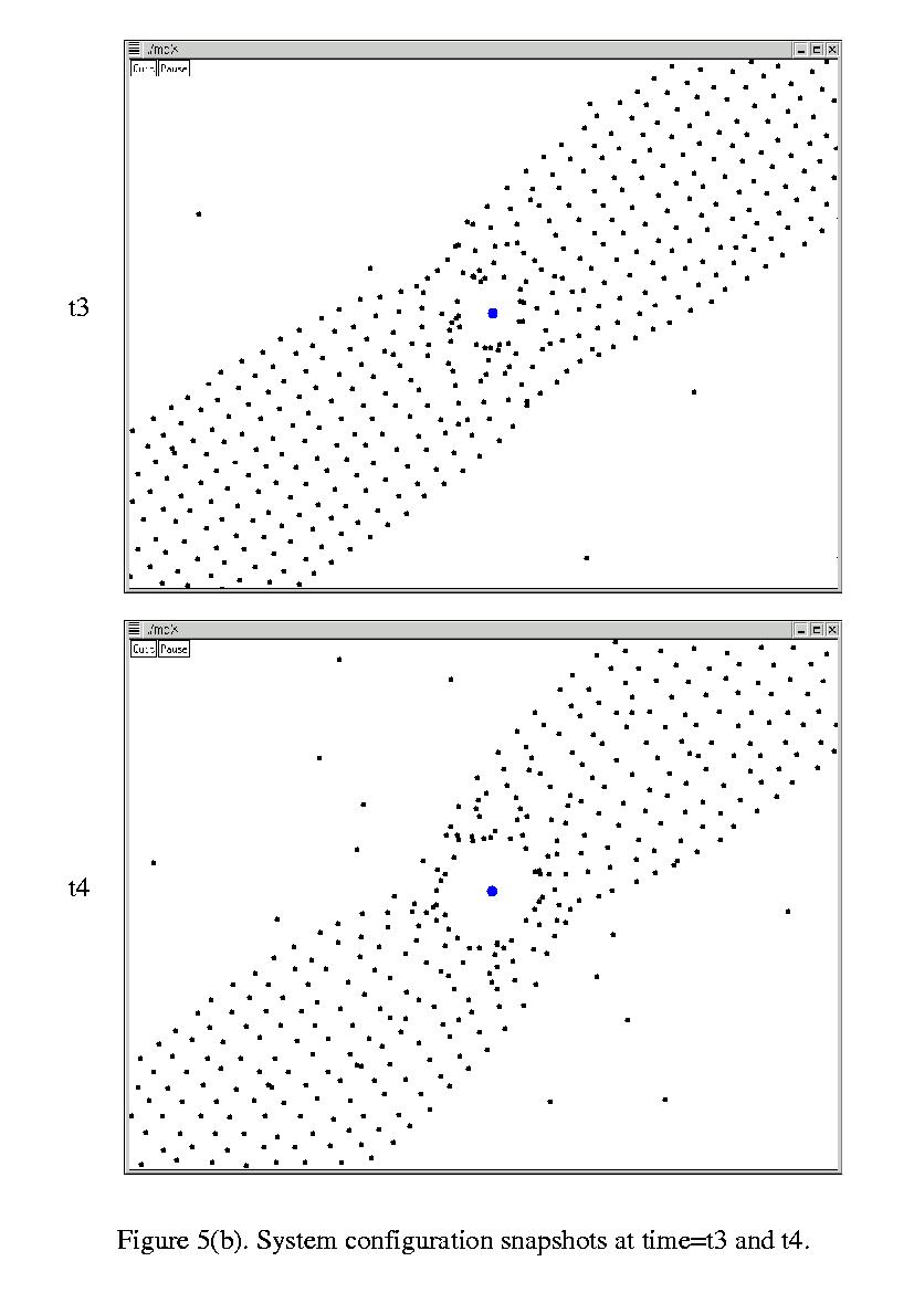
This simulation is used for the demonstration of parallel computing. With the combination of X window and MPI parallel programming library, we can see the evolution of the system during the simulation.
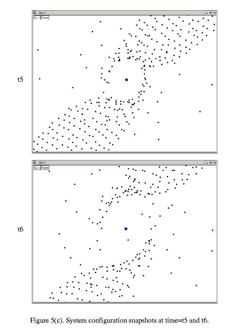
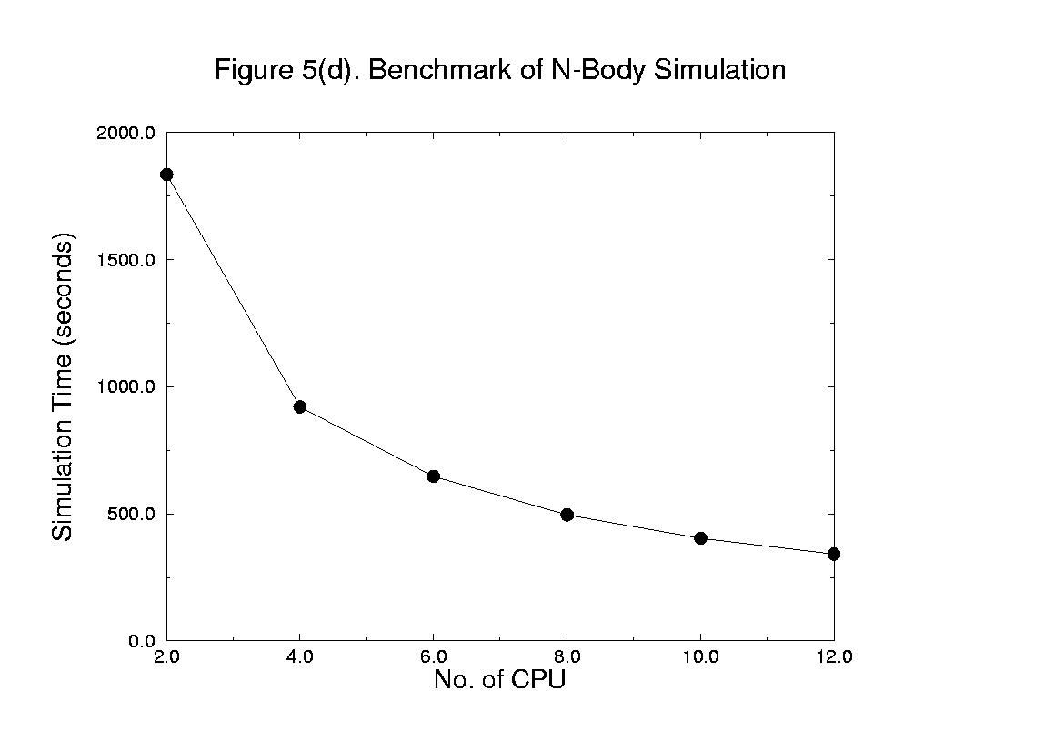
The inital configuration of the particles are arranged in a rectangle shape. There are total 1440 particles. All of them have the same mass except the one in the center which has the mass 1000 times bigger then others. The evolution of the system configurations are shown in (Figure 5(a), Figure 5(b), Figure 5(c)). The simulation time vs number of processor (CPU) is shown in (Figure 5(d)).
| length(byte) | time (sec) | Rate (MB/sec) |
|---|---|---|
| 1024 | 0.000955 | 8.578010 |
| 2048 | 0.001703 | 9.617846 |
| 4096 | 0.003105 | 10.555001 |
| 8192 | 0.006131 | 10.689284 |
| 16384 | 0.012167 | 10.772746 |
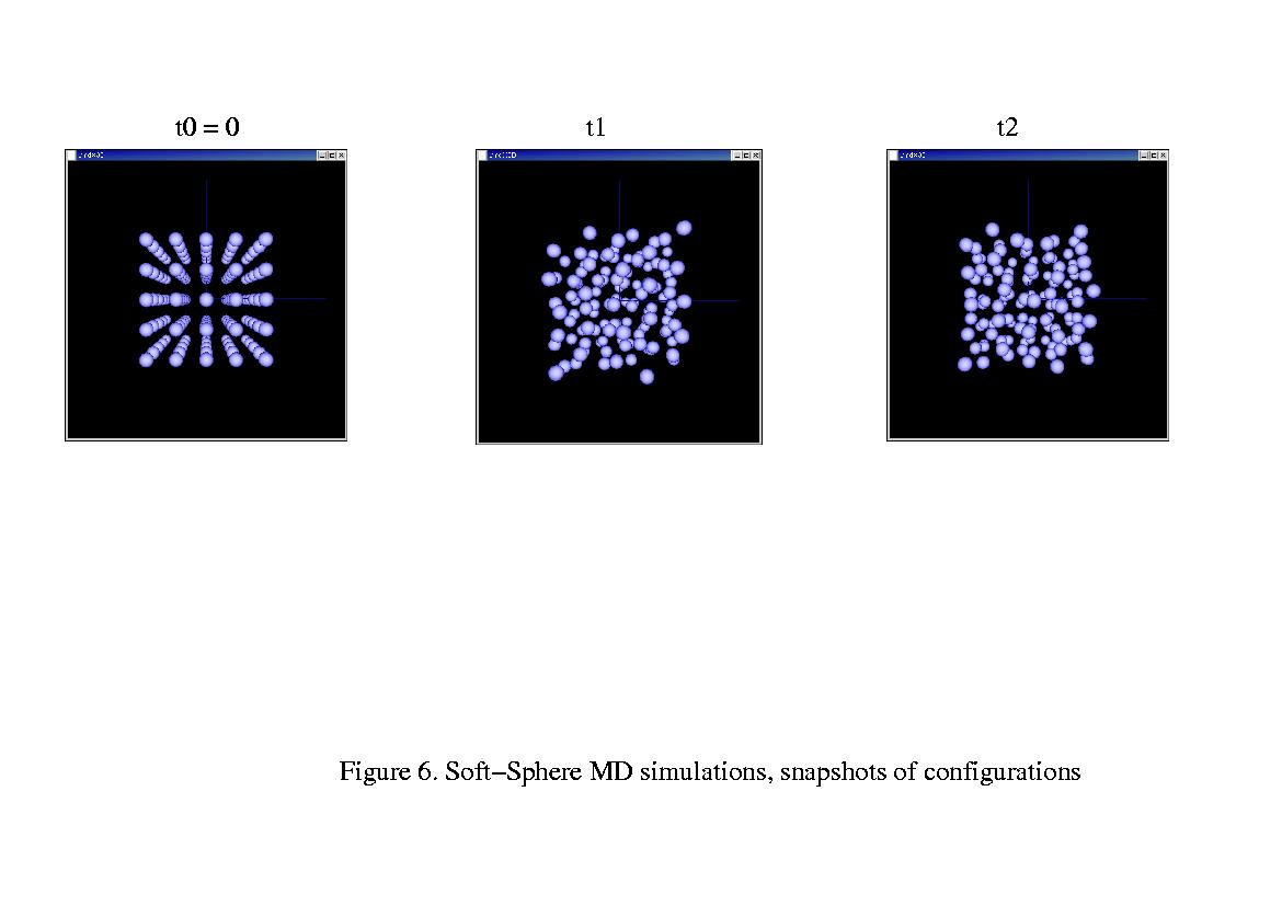
Basically, this example is the same as example 1 except the system is in three dimensional space. We use this example to demonstrate how to combine the simulation program with OpenGL library to generate 3D effects such as depth, shadow, lighting, etc. (Figure 6).
This simulation is used for the demonstration of 3D animation.
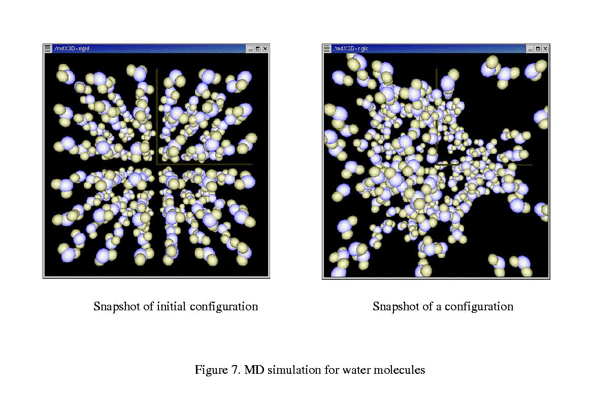
This example is the simulation of water molecule using rigid water model (TIP4P). The big sphere represents oxygen atom and the small sphere represents hydrogen atoms. We use this example to demonstrate the importance of visualization.
The initial position of each water molecule is arranged in the center of unit cube with randomly assigned orientation. After a while, we can see from the display window (Figure 7), the hydrogen bonds are formed between different water molecule.
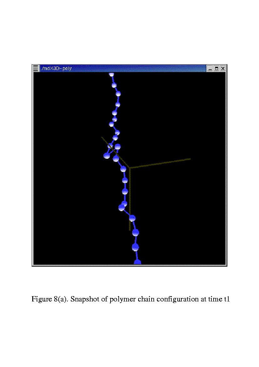
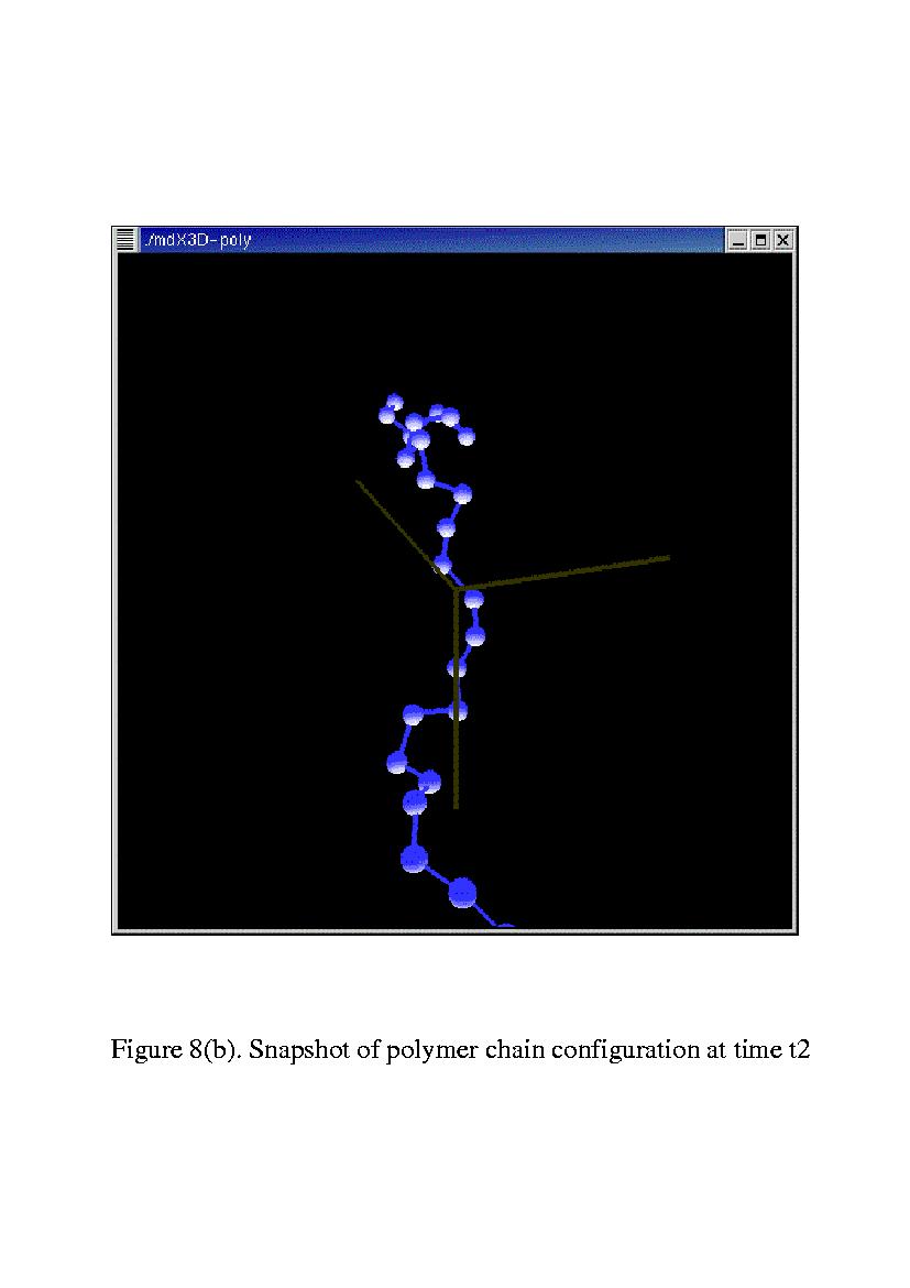
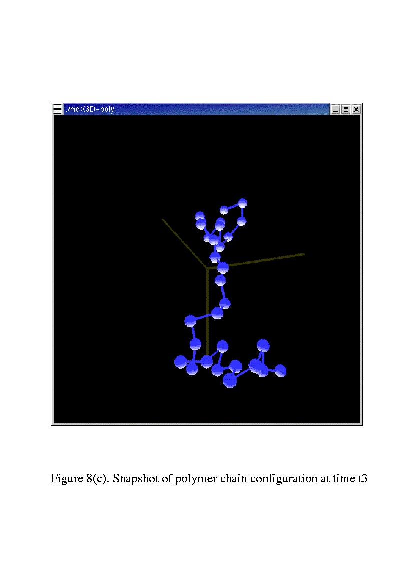
The purpose of this example is the same as in example 4. Through the real time animation we can see the folding process of a polymer in a soft-sphere solvent (Figure 8(a), Figure 8(b), Figure 8(c)).
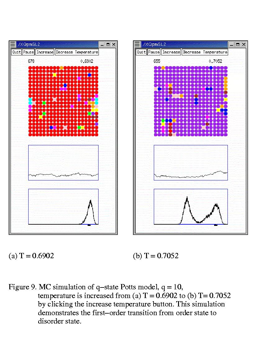
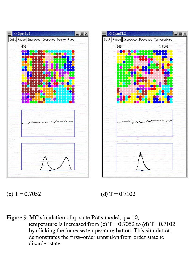
This example demonstrate the first-order phase transition of q=10 Potts model. We can decrease or increase the temperature to see the transition from order states to disorder states of Potts model by clicking the "Increase" or "Decrease" button. (Figure 9(a)-(b), Figure 9(c)-(d)).
So far, we've built our own virtul laboratory totally relied on free software. We also demonstrate that it is possible to achieve visibility, interactivity, and high-performance computing capabilities from scratch. The motivation of this project is not try to compete with some excellent commercial or academic MD packages, instead we try to get familiar with our research tools through the building process. We regard this project as an infrastructure for future complex problem studies and we will continue to improve it.